
Excel Formulas for Google Ads Editor and Ad/Keyword Imports
I’m sometimes asked in the office to help with Excel stuff, usually, it’s the same stuff over and over; So, here’s a list of the common basic Excel stuff I’m asked to help with and hopefully an explanation of how it works and how it’s useful for Google Ads.
I like to use spreadsheets and Editor to upload new ads and keywords as it’s two steps away from a live account and spending loads of money; Excel doc > AdWords Editor > Post to Google Ads live account, that’s ample time to spot any errors and correct. It’s also very handy and a lot quicker when working in bulk. Also, you have a dated backup of all the actions you’ve completed and a chance to send to whoever for adjustments/compliance.
The file used in all the examples is available here and can be used to create a basic account structure with ads for any beginner account creators.
Concatenate
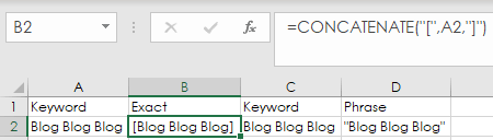
=CONCATENATE(“[“,A1,”]”) – this will return square brackets around anything in cell A1
You can concatenate anything to anything with this formula, so if you wanted to add text from A1 to A2 with a space in between you would use (A1,” “,A2). There aren’t too many rules to follow with this function as you can add things in any order, you can reference cells, or input text directly with quotation marks.
Concatenate can be used for exact, phrase, and broad match modifier keywords. Anything you put in quotations will be outputted, so this is useful for making ad customisers too.
Char(34)
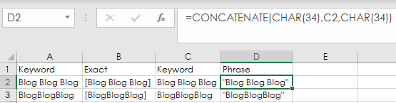
This one isn’t so much an Excel tip as a useful piece of information to be used alongside the concatenate formula. Char(34) is “ in computer speak.” If you try to add some keywords as phrase match with concatenate you might try this; =CONCATENATE(“””,A1,”””) – but Excel won’t have any of it! =CONCATENATE(char(34),A1,char(34)) works a treat though. There’s a full list of other ASCII characters here for any other special symbols or characters you’re trying to use that might be flagging up an Excel error.
Substitute
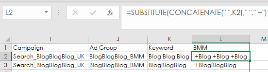
=SUBSTITUTE(CONCATENATE(” “,K2),” “,” +”) – This one looks a lot more complicated than it is, but all it does is add a space character at the start (So Excel doesn’t think we’re trying to do a sum), and then substitutes a space “ “ with a space and a plus “ +” for broad match modifiers.
Length
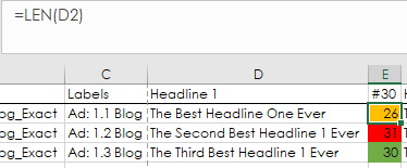
=LEN(A1) – will count and output the number of characters in cell A1 in a numerical value including spaces
Pretty simple and great for character limits in Google Ads (30 characters for your headlines, 90 for your descriptions, 15 for paths, 25 for callouts, 25 for link text in sitelinks)
Conditional Formatting
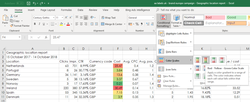
Another helpful tool in Excel is the conditional formatting feature. This is handy for graphically identifying cells above a certain character limit (as seen above and in the downloadable spreadsheet), or easily analysing large quantities of data. I tend to use either colour scales or data bars.
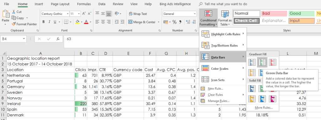
To add conditional formatting to your worksheet select the cells you’d like to apply it to, then on the home ribbon at the top of the workspace click the conditional formatting option, and select the type of conditional formatting you want.
Colour Scales
Data Bars
Find & Replace with *
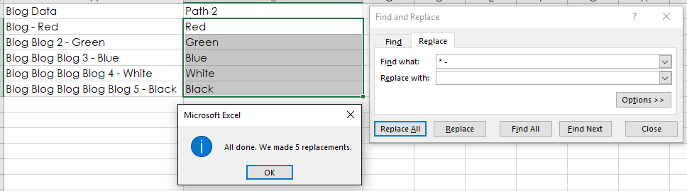
Find and replace is useful (CTRL + F) but using * is something that’s saved me loads of time and I don’t think many people use it or even know that they can. For example, I have a large amount of data at varying lengths in a spreadsheet, but I’d like the last word to go in my Path 2 for an ad.
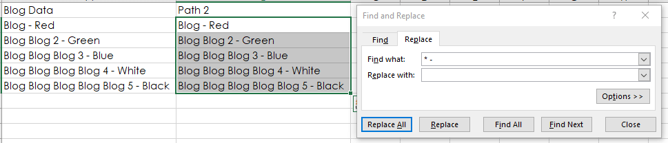
You could try writing a long winded Excel formula to find the first “ “ from the right and remove everything else left of that, or you could just type “* – ” in ‘Find what’ and “” in ‘Replace with’ and this will quickly find the first instance of “ – “ and remove everything before. The star will ignore/select everything before or after a character or selection of characters in the cells you select, then replace that with what you add in ‘Replace with’
VLookup
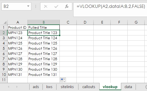
=VLOOKUP(A2,data!A:B,2,FALSE) – This looks up the content in cell A2 to content in a different sheet called ‘data’ in columns A and B, and then will return anything matching from cell A from column B (which is what the 2 is for, if you wanted to output anything from a third column C you’d add 3 to that formula), false means it was to match the content exactly.
Sometimes you’ll have two sheets of data with some information on that you’d like to merge (an example would be a product feed and then the data for your shopping campaign in Google Ads – Google doesn’t show you the product titles, so you might want to merge that data together using the ID/MPN. Another example would be a stock sheet against conversions or bids), if you have one universal identifier you can use Vlookup to match one document column to another.
Proper/Lower
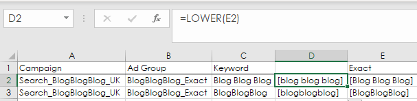
=LOWER(E2) – Lower will make all characters in a cell lowercase
=PROPER(E2) – Proper will make the first character of each word uppercase
=UPPER(E2) – Upper will make all characters in a cell uppercase – I don’t really use this one at all
Handy for if you like your keywords lowercase but your ad groups camel case.
Conclusion
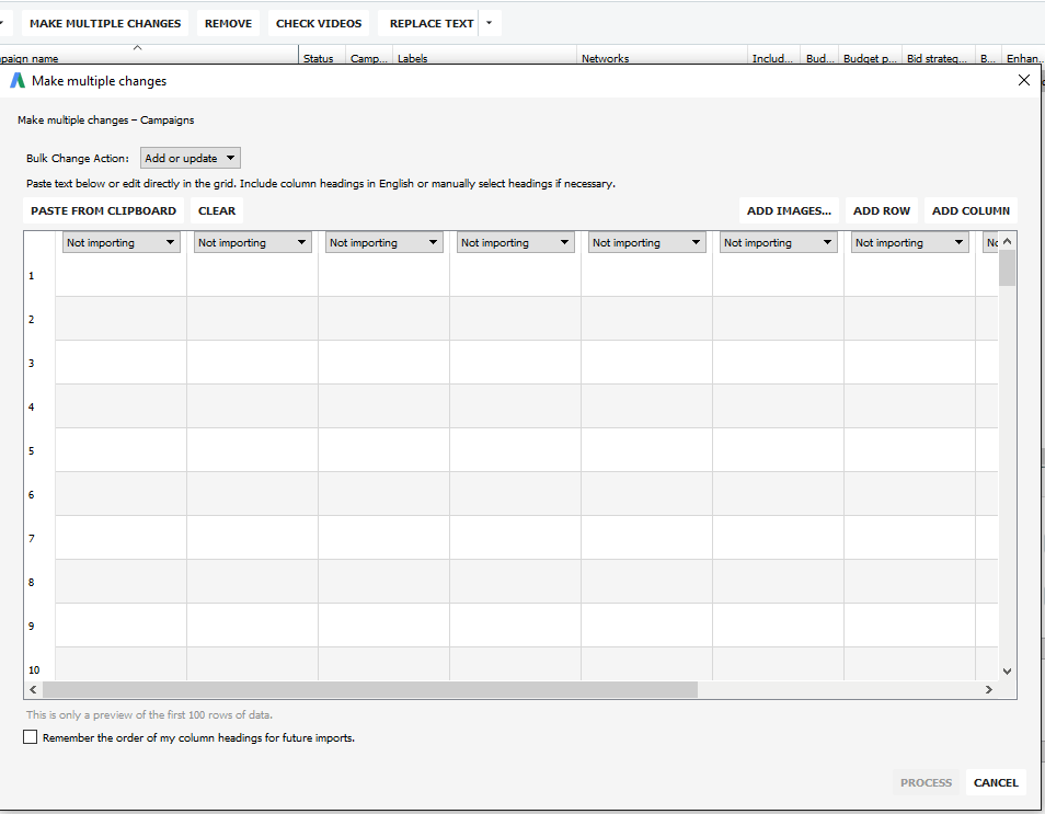
Microsoft Excel is a powerful tool for a many things, including Google Ads. With the above guide and spreadsheet, you should easily be able to create a beginner search campaign ready for import, the only additional requirement would be to export/copy the columns you require and paste them into a .csv file for uploading. Some of the guys in the office use the ‘Make multiple changes’ – which allows you to paste straight from the Excel document into Editor without having to make a separate file.
If you’re having trouble or would like something a little more advanced, get in touch! Either way, it’s great to have some input or a few USP ideas within ad copy to build from, so it’s worth having a go at populating a few cells yourself beforehand.